- Part 1: Using a queue
- Part 2: Sorting
- Part 3: The observer pattern
- Part 4: Go channels
This post is the second in a series, exploring a random assortment of techniques, data-structures etc. Each of which can be used to solve a puzzle from the 2015 edition of Advent Of Code, namely the first part of Day 7: Some Assembly Required.
See Part 1 for details on Advent of Code in general, as well as a summary introduction to the puzzle itself.
In this post we’ll take a look at how we can use sorting to solve the issue of instructions having arbitrary ordering in the input. We’ll be using Ruby again so we can do some run-time comparisons with the Queue based solution from Part 1.
Sorting
In computer science sorting usually means ordering elements of a list or an array in a lexicographical or numerical manner. E.g. for a random list of numbers, a sorted version could look like so:
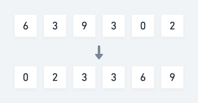
Each element compared to the next follows the relation a ≤ b. For numbers this relation is trivial because it has a strict mathematical definition. For words and letters it’s much the same, as each can be boiled down to a numeric representation as well.
In our case however each instruction isn’t necessarily directly comparable. Let’s take two random instructions from my input as an example:
fs AND fu -> fv
bz AND cb -> cc
If we just look at these two instructions, there isn’t any meaningful way that we can say that one should be ordered before the other. The relation between the two is simply lacking context.
Looking at each instruction individually however, we can reason about the relation between individual wires instead.
If we formulate the relation as depends on, for the above two instructions, we can say that fv depends on fs and fu, and that cc depends on bz and cb.
This should be enough to create an ordering definition that makes it possible to sort all instructions in a way where they can be carried out from top to bottom.
An instruction A with a lefthand side reference to a wire X depends on an instruction B with a righthand reference to a wire X.
As an example, the instruction ff AND fh -> fi depends on the instruction et OR fe -> ff. This means we must place the former after the latter in the the list of instructions.
Solution
The idea of this solution is that by re-ordering the instructions according to the above definition beforehand, we can then carry them out one by one, as is, and any wire will always have a signal by the time we reach an instruction that references it.
As in Part 1, we keep track of the overall state of the circuit in an associative array, which maps the name of a wire to its current signal value. Additionally in this version, we keep a list of wires which have resolved dependencies, which will form the decision basis for the ordering of sorted instructions.
The solution has three separate parts. Seeding, extraction and execution. Here’s the pseudo algorithm:
Outline
- Find the instructions that has no dependencies and use them to seed the sorted collection.
- While there’s still instructions left:
- Find the ones with resolved dependencies, extract and append them to the sorted collection.
- Execute the sorted instructions from top to bottom and store wire signals along the way.
- Print out the value of desired target wire.
Here’s the Ruby source:
Note: We have to do the same kind of bounding as in Part 1, in order to maintain 16-bit values throughout .
On lines 17-21 we do the initial seeding. Ruby has a .partition method which divides an enumerable into two new arrays based on the value of a predicate for each element.
We use this to separate all the instructions which we know have no dependencies, from the ones that have. Namely the instructions that directly assigns a signal to a wire. For each matching instruction we append the name of the output wire to the list of resolved wires, so we can use it for lookup later.
Lines 23-54 is really the meat of the program, and consists of an outer loop and an inner loop in the form of another .partition. The idea is pretty much the same as with the initial seeding, except this time we keep going until we’ve moved all remaining instructions into the sorted collection.
On each iteration of the outer loop, we pluck some subset of instructions which all have resolved wire dependencies and move them to sorted ones. At the same time we mark the output wires of those instructions as resolved as well.
Finally on lines 56-75 we carry out each sorted instruction and update the wire signals on the circuit as we go.
Input is again read from stdin, so the program can be run like so:
$ ruby 7p1-sort.rb < 7.inRun-time analysis
As with the Queue solution, I’m going to disregard regex matches and hash lookups, since they mostly likely are not the dominating factor.
Let’s look at each separate part of the program. Seeding and execution each runs through the list of instructions once yielding a O(n) + O(n) = O(n) run-time.
The most work is obviously done in the extraction part where we have a nested loop.
The outer loop is not bounded strictly by n, since we’ve already extracted some amount m of seed instructions. At the same time we extract some amount o of instructions each iteration, so the outer loop will never run n - m iterations because o > 0. Inversely the inner loop will pluck more and more instructions, due to more resolved wires. This makes o grow monotonically with each iteration of the outer loop.
However, since we cannot know for certain exactly how many instructions are extracted on each pass, we have to fall back on knowing that at least one instruction will be. This is yields the same familiar progression as in Part 1:
n + (n - 1) + … + 2 + 1
Good old O(n^2). That means we can throw out the lesser O(n) run-times of the seeding and the execution part.
We’re not quite done yet though. Inside that inner loop hides another lookup. Every time we test if a wire has been resolved, we do so by using .include. Which is most likely an O(n) linear search operation.
That means the final run-time complexity is O(n^3).
I’m sure there’s some tricks to make this approach more viable, but I’ll leave that up to the astute reader.
Still the output is small enough that the programs runs fast:
$ time ruby 7p1-sort.rb < 7.in
Signal ultimately provided to wire a: 16076

real    0m0.329s
user    0m0.260s
sys     0m0.051s
If we consider the running time of the Queue based approach, 0m0.225s, this is almost 50% slower by comparison however.
Memory usage
We’ll re-use the profiling approach from Part 1 and from that we can see the following allocations:
$ ruby 7p1-sort.rb < 7.in | head -3
Signal ultimately provided to wire a: 16076
Total allocated: 15.38 MB (248603 objects)
Total retained:  60.86 kB (1022 objects)
Again the sorting based approach takes a hit. It allocates about 4.3x the number of objects and uses about 3.3x the amount of memory compared to using a Queue.
Looking at which classes take up the most amount of memory this time around we get:
allocated memory by class
-----------------------------------
   7.10 MB  String
   5.89 MB  MatchData
   2.38 MB  Array
  14.43 kB  Hash
   72.00 B  Thread::Mutex
It’s not entirely surprising to see MatchData high up the list again, since we’re now doing the Regexp#=== pattern for the case statements in two different places.
I was a bit surprised at exactly how much String data was being allocated, so taking a look at another section of the MemoryProfiler output reveals that the most memory is allocated at the following lines:
allocated memory by location
-----------------------------------
   5.58 MB  7p1-sort.rb:31 (:27)
   2.07 MB  7p1-sort.rb:37 (:33)
   1.76 MB  7p1-sort.rb:41 (:37)
   1.31 MB  7p1-sort.rb:45 (:41)
   1.03 MB  7p1-sort.rb:47 (:43)
The line numbers are slightly off, compared to the version in the above gist, because that one doesn’t include the lines for MemoryProfiler. The ones in parenthesis correspond to the gist version.
The top offender is where we split an instruction into an expression and an output part on line 27. The other four are all MatchData from the regex matches in the following case block. It does make sense though, since these are all part of the inner loop.
All in all this approach is definitely a step back performance wise, compared to the Queue based solution.
In the next post we’ll take a look at a solution based on the observer pattern, which entirely sidesteps the issue of arbitrary instruction ordering, by managing dependencies as observers. Part 3.